Engineering Complexity and Community Friction
Joint predictors of high-speed rail cost: a reference-class analysis of 69 international lines, scored blind to cost, with cost predictions for the ALTO corridor.
This edition replaces the Initiative’s April 2026 analysis. Project costs now come from the NYU Transit Costs Project high-speed rail dataset, the source the Parliamentary Budget Officer used in its 1 October 2026 cost analysis (RP-2627-009-C), converted to 2024 Canadian dollars on PBO’s basis. The reference class grows from 16 projects to 69 lines in 21 countries, and every line was re-scored on both indices with cost information excluded.
The results are more modest than in April. The joint model now explains 42 % of cross-project cost variance, not 90 %, and engineering complexity, not friction, is the stronger predictor. The April figures on this page have been replaced throughout.
Both indices predict cost. Scored blind to cost on 69 lines, engineering complexity (ECI) and community friction (CFI) together explain 42 % of the cross-project variance in log-cost per kilometre. Both are statistically significant (ECIw p < 0.001; CFI p = 0.011). Engineering is the stronger: alone it explains 36 %, friction 10 %.
Friction adds explanatory power to a replication of PBO’s model. Added to PBO’s variables (tunnel and elevated shares, start year, region), each 10 CFI points is associated with about 13 % higher cost (p = 0.002). The effect holds without HS2 and California, without China and Japan, and within Europe.
ALTO prediction. The CRI multivariate model gives $191 million per kilometre at the projected CFI of 65, or $163 billion on PBO’s 850 km route, with a wide 95 % prediction interval of $48–547 billion. The probability of delivery at or below the Government’s $90 billion is about 17 %. The replicated PBO model gives $73 billion at European cost efficiency, and $115 billion with friction added.
Friction is the part of the prediction that can still change. If ALTO’s friction stays at today’s 43 rather than rising to the projected 65, the CRI multivariate prediction falls from $163 to $129 billion, about $34 billion lower.
What the revised analysis finds
All costs are 2024 Canadian dollars on PBO’s basis and cover civil works, systems, stations and overheads, excluding rolling stock and financing. Predictions are model-based estimates, and the intervals around them are wide.
Engineering complexity and community friction
Two instruments developed by the Initiative provide the input variables. Neither has been externally peer-reviewed. Both rubrics are unchanged from April.
The Engineering Complexity Index (ECI)
The ECI scores six physical engineering dimensions from 1 (routine) to 5 (extreme) against published anchor descriptions. The scores are weighted and combined into a composite, ECIw, on a 20-to-100 scale.
| Dimension | Weight | 1 · Routine | 3 · Moderate | 5 · Extreme |
|---|---|---|---|---|
| Geotechnical conditions | 20 % | Competent uniform ground | Mixed conditions, localised complications | Leda clay, extensive karst, permafrost |
| Major structures | 20 % | Predominantly at grade | 10–25 % tunnel or viaduct | Over 50 % tunnel or viaduct |
| Topography and alignment | 20 % | Flat, relief under 100 m | Significant relief or tight urban alignment | Mountainous, relief over 500 m |
| Hydrology and drainage | 15 % | Minimal watercourse crossings | Several major crossings, localised wetland | Dominant hydrological constraint |
| Infrastructure interfaces | 15 % | Rural, greenfield | Significant urban segments, utility relocation | Dominant urban and interface complexity |
| Climate and environmental loading | 10 % | Mild, negligible freeze-thaw | Substantial winter design, freeze-thaw cycling | Extreme combined loading |
ECI rubric. Full scoring descriptors are in Appendix A of the report.
How ALTO scores. On the Initiative’s scoring, the southern ALTO corridor scores ECIw = 77. It scores high on three dimensions at once: geotechnical conditions on the Canadian Shield, hydrology crossings, and freeze-thaw climate loading.
Geotechnical 5 reflects Leda clay, karst, Frontenac Arch bedrock exposure and the freeze-thaw regime; hydrology 4 reflects the Moira, Napanee and Salmon River crossings. Across the 69 reference lines ECIw runs from 34 to 87, with a mean of 63; nine lines score higher than ALTO. ALTO’s scores are carried over from earlier work and were not re-assigned under the blind protocol. On the blind scorers’ conventions its structures score would be 3 rather than 4, giving ECIw = 73.
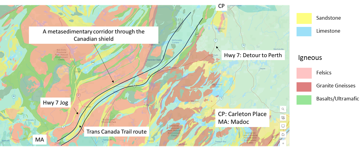
Geology along the southern ALTO corridor between Carleton Place (CP) and Madoc (MA). Source: CRI geotechnical brief.
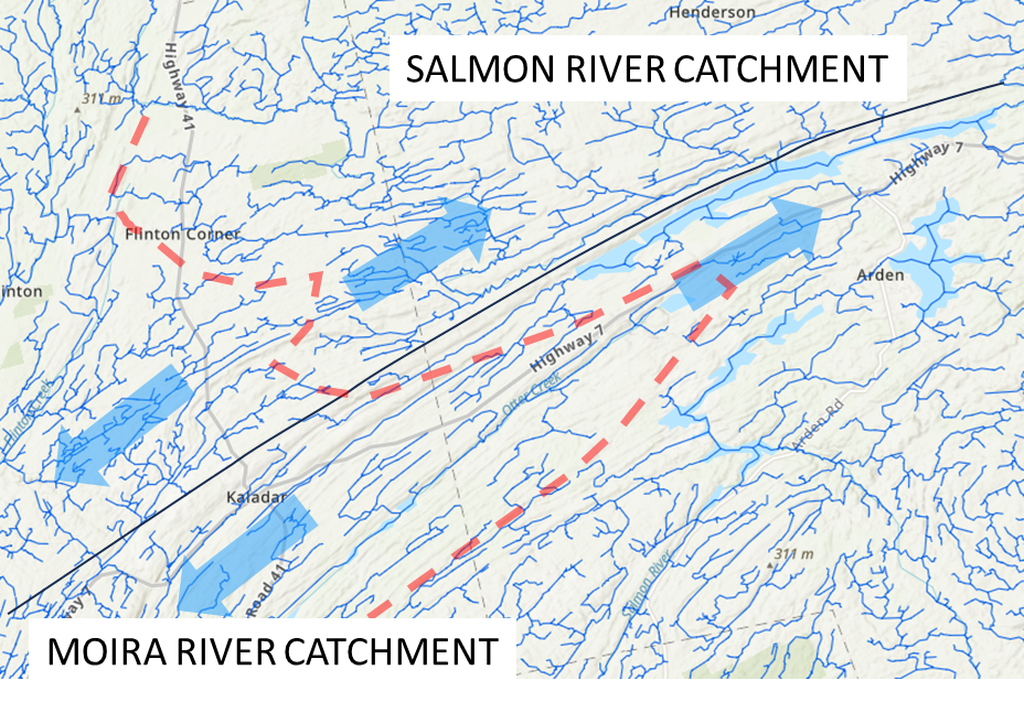
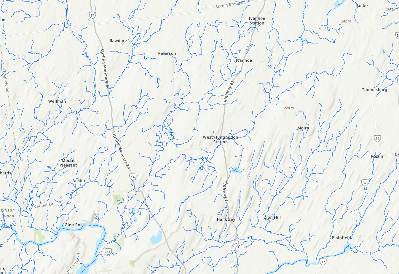
The Salmon River (left) and Moira River (right) catchments, each crossed by the southern route through mapped wetland and headwater systems.
The Community Friction Index (CFI)
The CFI measures the sociopolitical resistance a linear project generates along its corridor. It has five components, each scored 0–20 from the documentary record against a 20-indicator rubric and summed without weighting to an aggregate of 0–100. For this edition, any event whose subject was the project’s cost (budgets, overruns, value for money) was excluded from every component.
1 · Public opposition intensity
Scale, organisation and reach of grassroots opposition: objections, community groups, coalitions, media coverage, mobilisation.
2 · Legal challenges filed
Formal legal activity against the project or its approvals: pre-action letters, tribunal applications, judicial review, injunctions, constitutional and Indigenous-rights litigation.
3 · Forced route changes
Alignment, station or scope changes made under community, regulatory or political pressure.
4 · Environmental and NGO opposition
NGO engagement, from routine submissions through species-at-risk triggers, environmental litigation and regulatory intervention.
5 · Political controversy
Inter-party, inter-governmental and intra-caucus contest over the project, other than over its cost.
| CFI range | Band | Reference lines in this band (blind scores) |
|---|---|---|
| 0–25 | Low | Most Chinese, Japanese, Turkish and Spanish lines; LGV Sud-Est (11), Madrid–Seville (11), Taiwan HSR (17) |
| 25–45 | Moderate | LGV Nord (29), LGV Atlantique (32), Florence–Bologna (38), Madrid–Barcelona (42), Gardermobanen (42); ALTO today (43) |
| 45–65 | High | HS1 (50), California IOS (50), VDE 8 (55), HSL-Zuid (56), Cologne–Frankfurt (57), Rail Baltica (59), Lyon–Turin (64), Gyeongbu Phase 2 (64) |
| 65–85 | Very high | HS2 Phase 1 (68); ALTO projected (65) |
| 85–100 | Extreme | No reference line once cost-driven controversy is excluded |
CFI bands, with reference lines placed by their blind scores. Bands are interpretive; the regressions use the continuous score. Source: report Table 4.
Why the scores were re-assigned
The April scores were assigned by a scorer who already knew each project’s cost and history. That tends to make indices track outcomes and overstate their predictive power. This edition uses a blind protocol. Scorers did not look up or use any information on cost, budget, cost per kilometre or overruns. Engineering was scored on the physical characteristics of the costed section. Friction was scored from the documentary record, excluding any event whose subject was cost. Where evidence was equivocal, the lower score was used, and each line carries a confidence rating.
The scores were assigned by AI research agents working from the published rubrics and the public record, one pass per line. No second scorer has yet checked them. Every score is published in the report with its evidence and sources so that any of them can be checked and revised. Blindness cannot be complete, since a scorer may know a famous project’s reputation.
| Measure | April 2026 16 projects |
16 projects sourced costs |
October 2026 69 lines, blind |
|---|---|---|---|
| R², ECIw alone | 0.57 | 0.54 | 0.36 |
| R², CFI alone | 0.81 | 0.40 | 0.10 |
| R², ECIw + CFI | 0.90 | 0.66 | 0.42 |
| CFI p-value, ECIw + CFI | < 0.001 | 0.054 | 0.011 |
| Completion year | p = 0.83 | p = 0.14 | p = 0.001 |
| ALTO, $M per km | $142 | $229 | $191 |
| 95 % interval spans a factor of | 3.5 | 19 | 11 |
Key results at each stage. The middle column re-ran the April models with Transit Costs data and the April scores. Source: report Table D-1.
Blind friction scores track the April scores reasonably closely (r = 0.74) but average 9 points lower, mostly for projects whose controversy was about cost: HS2 falls from 92 to 68 and California from 78 to 50. Engineering scores changed more (r = 0.47). California moves most, because its costed section crosses the flat Central Valley.
Engineering complexity is the strongest single predictor
Engineering alone explains 36 % of cross-project cost variance, more than friction or completion year. The fit implies roughly 42 % higher cost for every 10 ECIw points, close to the 49 % reported in April, with more scatter around the line. Applied to ALTO’s ECIw of 77, engineering alone predicts $129 million per kilometre.
Cost per kilometre against ECIw for the 69 reference lines, coloured and shaped by region; log scale. The dashed line is the OLS fit. The ALTO marker shows the joint prediction of $191 M/km at ECIw 77 and CFI 65. Hover a point for its line and scores. Data: report Appendix B.
As in April, the U.K. and U.S. projects (HS2, HS1 and California) sit above the engineering line, and several Spanish and French lines sit below it. Factors beyond ground, structures and terrain affect cost, and the rest of the analysis tests whether community friction is one of them.
On its own, friction is a weak predictor
With cost-driven controversy removed from the record, friction alone explains 10 % of cross-project cost variance, not the 81 % reported in April. The fit implies roughly 15 % higher cost per 10 CFI points, against 38 % in April. Applied to ALTO, friction alone predicts $137 million per kilometre at the projected CFI of 65 and $101 million at today’s 43.
Cost per kilometre against CFI for the 69 reference lines; log scale. The dashed line is the OLS fit. Data: report Appendix B.
Why the April result did not hold
Cost-driven controversy is out. Excluding opposition about budgets and overruns lowers the scores of the costliest projects most.
The sample is broader. The expanded class includes many higher-cost Asian lines with little documented friction, such as Beijing–Tianjin, Hokuriku and Taiwan HSR, which weakens the simple association. Opposition on some of these lines may be under-recorded.
Friction’s contribution appears once engineering and region are controlled for, as the next two findings show.
Together, ECIw and CFI explain 42 % of cost variance
Both coefficients are statistically significant: ECIw (p < 0.001) and CFI (p = 0.011). Each 10 ECIw points is associated with about 39 % higher cost and each 10 CFI points with about 11 %. The standardised coefficients are 0.57 for engineering and 0.25 for friction, reversing the April balance (0.35 and 0.70). Engineering adds 32 points of R² over friction; friction adds 6 points over engineering. The two indices are almost uncorrelated (r = 0.13; variance-inflation factor 1.02), so their separate effects can be estimated cleanly. This model is referred to below as the CRI multivariate model.
Observed cost per kilometre against the CRI multivariate model’s prediction for the 69 reference lines. Points above the dashed line cost more than the model predicts. The shaded band marks ±0.25 log-units (about ×1.8); the largest misses are labelled. ALTO sits on the line by construction. Source: report Figure 2 data.
Influence. HS2 sits far above the fitted line. Excluding HS2 and California together lowers the friction coefficient in this two-variable model and it is no longer significant (p = 0.23); engineering is unaffected. Finding 4 shows that the friction effect does not depend on these two projects once the regional cost level is controlled for.
Completion year now matters. The April edition found that completion year added nothing once both indices were controlled for. On sourced data that no longer holds. Adding completion year raises R² to 0.51 (adjusted 0.49), and the year coefficient is equivalent to about +2 % a year in real construction cost per kilometre (p = 0.001), close to the start-year effect in PBO’s model. Both indices remain significant.
Share of variance in log-cost per kilometre explained by each specification (n = 69). Left: the Initiative’s index models, with the CRI multivariate model highlighted. Right: the replicated PBO model (tunnel and elevated shares, start year, region) alone and with the indices added. Source: report Appendix C.
An intuition: two factors, one price
A house’s price depends on both its size and its location. A rail corridor’s cost depends on both its engineering complexity, which is like the house, and its community friction, which is like the lot: the neighbours, the permits, the time spent before a shovel enters the ground. On the revised evidence the house matters more than the lot, with engineering carrying a little more than twice friction’s weight. But the lot still moves the price once the house is accounted for.
Friction adds explanatory power to a replication of PBO’s model
PBO explains cost with measured tunnel and elevated shares, construction start year and regional cost levels. Because its engineering variables are measured rather than scored, and it controls for region, adding the indices to it is the hardest test of whether they carry information PBO’s model does not already contain. Fitted to the same 69 lines, the Initiative’s replication reproduces PBO’s published results closely and explains 66 % of variance.
| Model | R² | Adj. R² | Key result |
|---|---|---|---|
| PBO model (tunnel, elevated, start year, region) | 0.660 | 0.627 | All engineering variables significant; U.K./U.S. ×4.8 |
| + CFI | 0.709 | 0.675 | CFI +13 % per 10 points; p = 0.002 |
| + ECIw | 0.696 | 0.661 | ECIw +20 % per 10 points; p = 0.009 |
| + ECIw + CFI | 0.721 | 0.684 | CFI p = 0.024; ECIw p = 0.11 |
The indices added to the replicated PBO model (n = 69). Source: report Table 8.
Each 10 CFI points is associated with about 13 % higher cost (p = 0.002), and the estimated U.K./U.S. premium falls from ×4.8 to ×3.4, so friction accounts for part of what the model attributes to region. Engineering complexity also adds on its own (p = 0.009), consistent with the ECI capturing ground and terrain conditions that tunnel and elevated shares miss; PBO’s report notes that its model does not capture Canadian Shield conditions. With both indices included, friction remains significant and engineering does not, partly because the ECI’s structures dimension overlaps the tunnel and elevated shares.
| Sample | n | ECIw + CFI per 10 CFI · p |
PBO + CFI per 10 CFI · p |
|---|---|---|---|
| All 69 lines | 69 | +11 % · 0.011 | +13 % · 0.002 |
| Excluding HS2 and California | 67 | +5 % · 0.230 | +13 % · 0.004 |
| Excluding China and Japan | 54 | +17 % · 0.005 | +12 % · 0.012 |
| Europe only | 42 | +10 % · 0.141 | +12 % · 0.017 |
| Friction confidence high or medium only | 35 | +9 % · 0.186 | +15 % · 0.014 |
Friction effect across subsets. “Europe only” omits the regional indicators. Source: report Table 8b.
Reading the robustness test
In the replicated PBO model the friction effect is stable, between +12 and +15 % per 10 points, and significant in every subset: without HS2 and California, without China and Japan (where opposition may be under-recorded), within Europe alone, and using only lines whose friction scores carry medium or high confidence. In the two-variable model the estimates are similar, but significance depends on the U.K./U.S. projects and on sample size. Friction is best estimated alongside a control for the regional cost level.
Out-of-sample check: Rail Baltica
Rail Baltica, an 870 km line through the Baltic states, is not in the Transit Costs dataset and was held out. Its blind scores are ECIw 52 and CFI 59, and its cost on the dataset’s basis is $54 million per kilometre. Fitted on the other 68 lines, every model’s 95 % interval contains that cost. The nearest is the PBO model ($55 M); the bivariate model gives $81 M and the PBO model with friction $90 M. Adding friction moves the prediction away from the actual cost: Rail Baltica is a high-friction line that has so far been relatively cheap per kilometre, on a route only about a third designed.
Today’s CFI of 43, and the projection to 65
ALTO’s friction score is taken from the Initiative’s friction note. It was scored from the documented record as of the April 2026 consultation deadline, after Bill C-15. At 43 it sits in the upper Moderate band, two points below the High threshold. Public opposition and political controversy are the largest components; forced route changes are limited by the Bill C-15 s. 98 CTA deeming provision. ALTO’s score was not re-assigned under the blind protocol, but it includes little cost-driven controversy.
Stated positions, as compiled by a community group
Organisations that have stated positions on the current ALTO plan include the Ontario Federation of Agriculture, Beef Farmers of Ontario, the National Farmers Union — Ontario, municipal councils, Conservation Authorities, MPs, MPPs, and community and business groups. The map below compiles those statements. It is reproduced here as part of the documentary record on which the friction score is based.
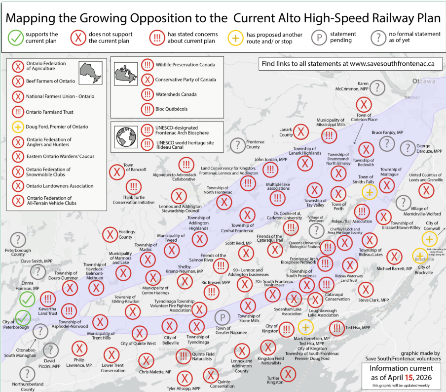
Documented stakeholder positions as of April 15, 2026. Graphic compiled by Save South Frontenac volunteers, a community group opposed to the southern route; links to the underlying statements are at savesouthfrontenac.ca. The Initiative has not independently verified each entry. The map records stated positions only.
Three scenarios from one baseline
The friction note projects three trajectories from today’s 43 to 2030. The mid-energy endpoint of 65 is the basis for the central cost prediction. These are scenario assumptions, not forecasts.
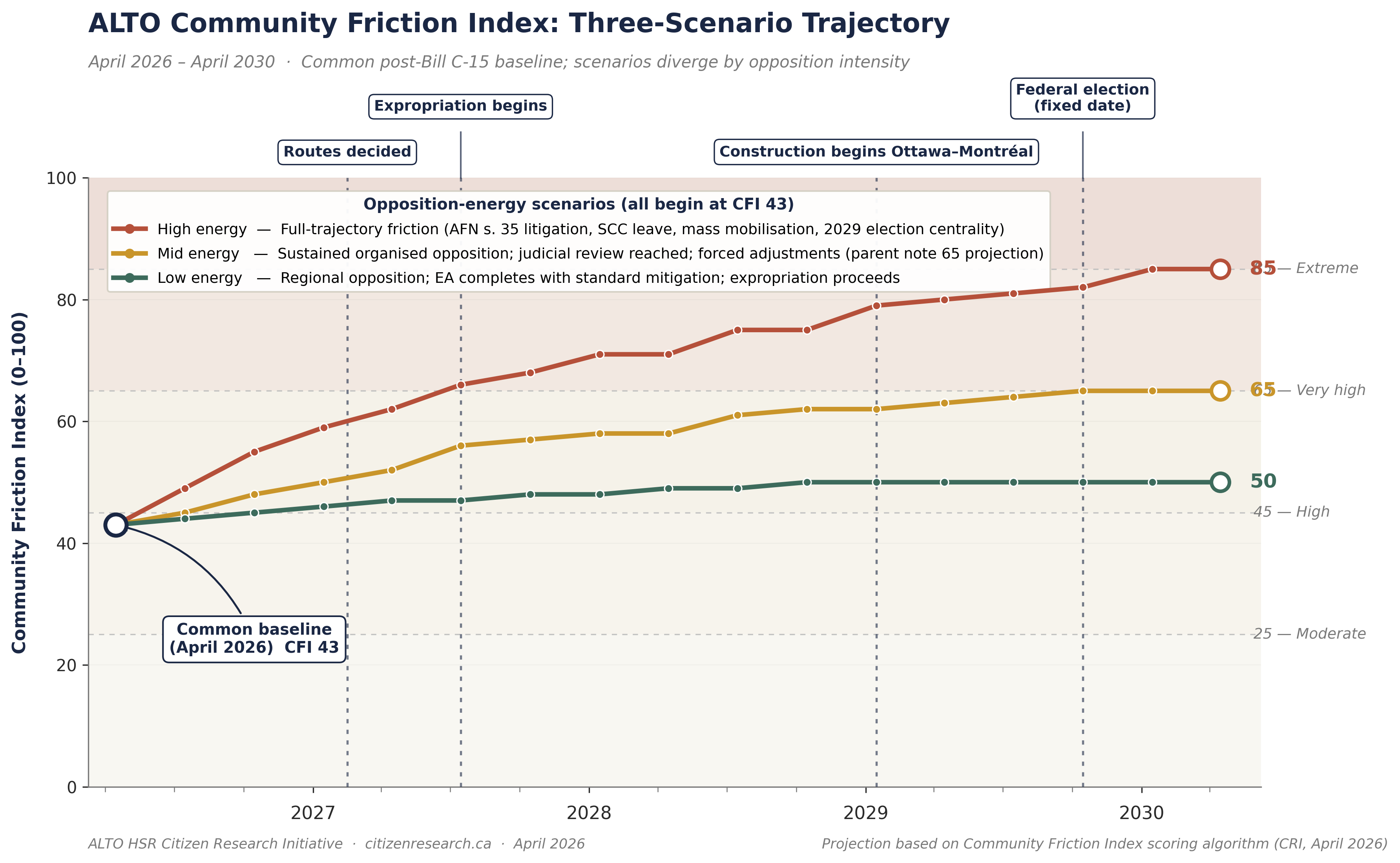
Three-scenario projection of ALTO’s CFI, April 2026 to April 2030. Source: CRI friction note.
Decomposed into its components, the mid-energy path is dominated by legal activity (+8) and route changes (+5), with political controversy +4, environmental +4 and public opposition +1. The scenario assumes that the s. 98 CTA deeming provision limits growth in the route component and that pressure moves instead to access-to-information requests, judicial review and constitutional avenues.
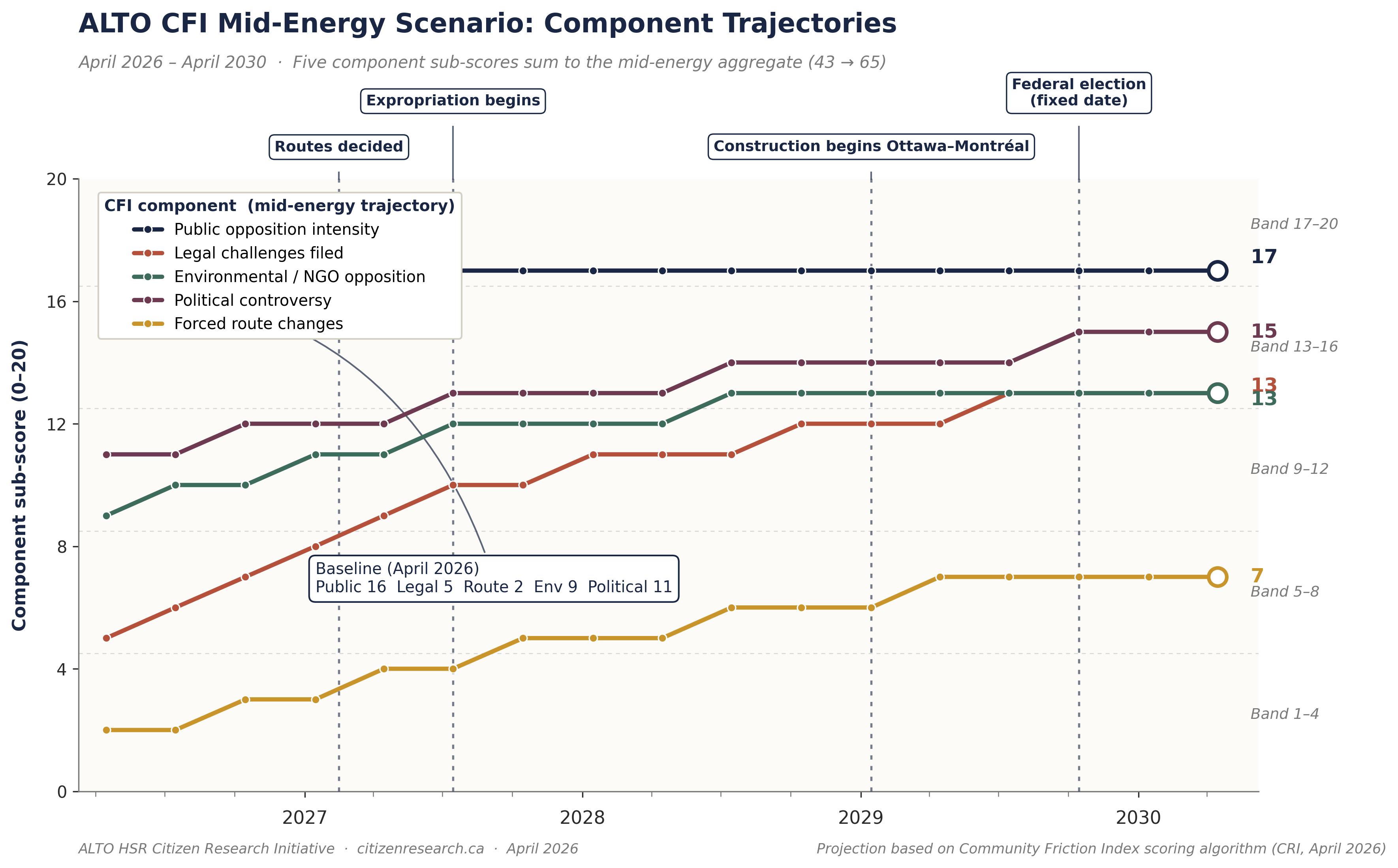
Mid-energy component trajectories, as projected in the friction note.
Conditions associated with rising friction
The megaproject literature and the friction note identify conditions associated with rising friction. They are listed here as general risk factors; their inclusion is not a finding that each one applies to ALTO.
At projected friction, every model with either index places ALTO above the stated range
The CRI multivariate model returns $191 million per kilometre at the projected CFI of 65, or $163 billion on PBO’s 850 km baseline route, and $151 million ($129 billion) at today’s CFI of 43. The Government’s stated capital cost is $60–90 billion, or about $71–106 million per kilometre on that route; PBO’s published estimate is $75–113 billion.
Medians on the log scale, 2024 CAD. Shaded: the Government’s $60–90 B, and the span to PBO’s $113 B upper bound. Not shown: the replicated PBO model at the U.K./U.S. cost level, $349 B. At today’s CFI of 43, the friction-only model ($86 B) and the PBO model with friction ($88 B) fall within the Government’s range. Source: report Table 9.
The replicated PBO model returns $73 B, close to PBO’s published $75 B, because it prices ALTO at European cost efficiency with no allowance for friction. Adding friction to it raises the figure to $115 B. Adding completion year to the CRI model raises its prediction to $237 B, because ALTO would be built later than most of the reference class. With the U.K./U.S. cost-level indicator switched on, the replicated PBO model gives $349 B. The CRI multivariate prediction sits between the European reference and that adverse case.
The 95 % prediction interval
Real projects scatter widely around any fitted line, so the interval is wide: $48 B to $547 B on 850 km, a factor of 11 (against 19 in the 16-project analysis). Allowing for that scatter, the expected (mean) cost is about $228 million per kilometre.
How likely is the stated range?
| Model | ≤ $60 B | ≤ $75 B | ≤ $90 B | ≤ $113 B |
|---|---|---|---|---|
| CRI multivariate model, CFI 65 | 5 % | 10 % | 17 % | 28 % |
| CRI multivariate model, CFI 43 | 10 % | 18 % | 27 % | 41 % |
| PBO model + CFI, CFI 65 | 9 % | 19 % | 30 % | 48 % |
| PBO model, replicated (Europe cost level) | 35 % | 52 % | 66 % | 81 % |
Probability that ALTO’s construction cost on the 850 km route falls at or below each threshold, from each model’s prediction distribution. Source: report Table 10.
Under the CRI multivariate model, the Government’s $90 B has about a one-in-six chance of being met at the projected level of friction, and PBO’s $113 B upper bound about 28 %. On the replicated PBO model alone, $90 B is more likely than not. Friction and engineering complexity, which PBO’s model does not score, account for the difference.
Friction is a measurable cost factor, and one that can change
These are statistical associations across projects, not proof that friction causes cost. Because cost-driven controversy was excluded from the scores, the association is less likely to reflect expensive projects attracting opposition than in the April analysis. Some reverse causation may remain: a line that takes longer can accumulate more friction. Engineering complexity is largely fixed by the route; friction is not. In the replicated PBO model, each 10 friction points avoided is associated with roughly 13 % lower construction cost.
Recommendations in the report
Limitations
Summary ledger
How each conclusion of the April 2026 edition fares on sourced costs and blind scores: